Presentation-Outline

Robotic Autofocus for Visual Inspection — Presentation Outline

Ratio-Based Velocity Control for Robotic Macro Imaging in Precision Manufacturing
Santoso, Acton, Back, Chen — MACS Lab, University of Washington

Target: ~15 min talk (~13 slides, ~1 min each). Bullets below summarize what to say per slide.

---

Slide 1 — Title & Motivation Hook

• Robotic autofocus algorithm for visual inspection in precision manufacturing
• Key claim: reaches optimal focus in < 25% of the time of exhaustive hill climb, while holding 2 mm accuracy on textured surfaces / 4 mm on smooth/reflective ones
• Works across multiple focus metrics and 9 materials with no recalibration

---

Slide 2 — Why Automated Inspection?

• Quality control is critical in aerospace / precision manufacturing: complex geometries, tight tolerances, variable composite materials
• Manual inspection is error-prone — humans miss up to 25% of defects in enterprise-scale tasks
• Automation is faster (< 40% of human inspection time), more accurate (+17%), and cheaper (~40% cost reduction per component)
• High-mix, low-volume sectors (aerospace) have been slow to adopt — motivates this work

---

Slide 3 — The Autofocus Problem

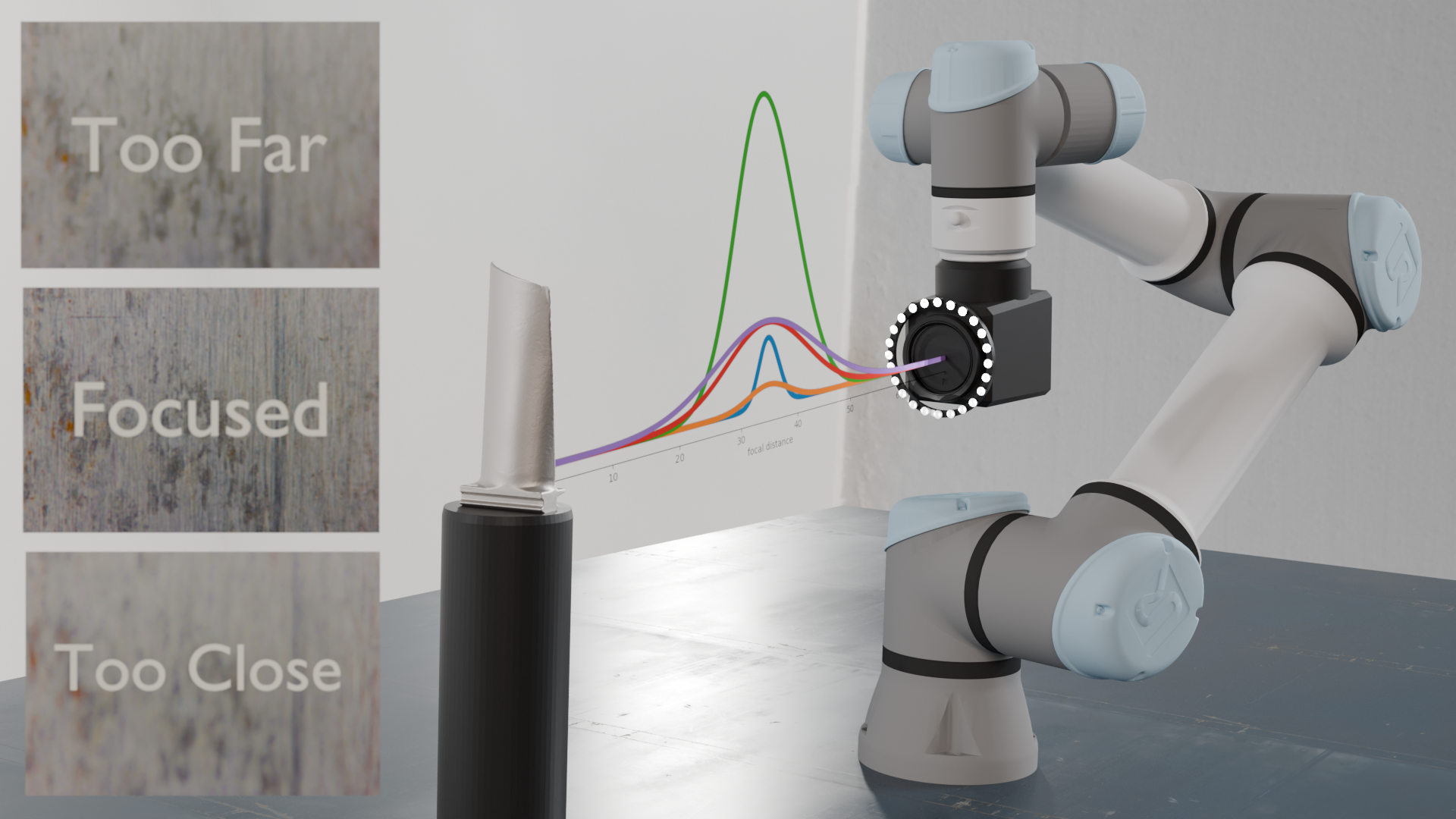
• Focus on visual inspection: low-cost, accessible; goal is consistently sharp images
• Core challenge: maintain accurate focus while preserving constant magnification
• Cannot use in-lens autofocus — it changes focal length → changes magnification → corrupts geometric data for downstream ML/defect detection
• Solution: focus by moving the robot arm, not the lens
• Shallow depth of field on a macro lens makes reliable autofocus essential

---

Slide 4 — Why Not Standard Optimization?

• Focus Value (FV) curve is non-smooth: extensive flat regions + a narrow peak
• Newton’s method: noise-sensitive, needs a good initial guess, fails in flat/non-smooth regions; no analytic gradient/Hessian for FV
• Bayesian optimization: assumes smoothness, needs per-object/environment tuning, struggles with flat regions and narrow peaks
• Neither delivers real-time, robust autofocus across diverse inspection scenarios

---

Slide 5 — Our Approach & Contributions

• A data-driven, ratio-based adaptive autofocus framework
• (i) Novel ratio-based robotic autofocus that works across multiple focus metrics & materials without recalibration
• (ii) Comprehensive evaluation of focus metrics under consistent conditions across materials
• (iii) High-precision demonstration: sub-mm on textured, 4 mm on smooth surfaces
• Repurposes ratio control (from mixing applications) — uses the ratio of focus values as the control input, so it’s metric-scale-agnostic

---

Slide 6 — Focus Value & The Three Metrics

• FV = image sharpness from high-frequency edge content; plotted vs. focal distance → bell curve, peak = optimal focus
• Variance of Sobel — robust to Gaussian noise, but lower sensitivity to fine edges
• Squared Gradient (SG) — more edge-sensitive, but can amplify noise
• FSWM (frequency-selective weighted median) — strong noise robustness + edge preservation, but computationally expensive
• Different strengths → motivates a system that adapts across metrics
• $FV={\sum }_{x,y}(G_x^2+G_y^2)$ for SG; FSWM uses weighted-median filtering then variance

---

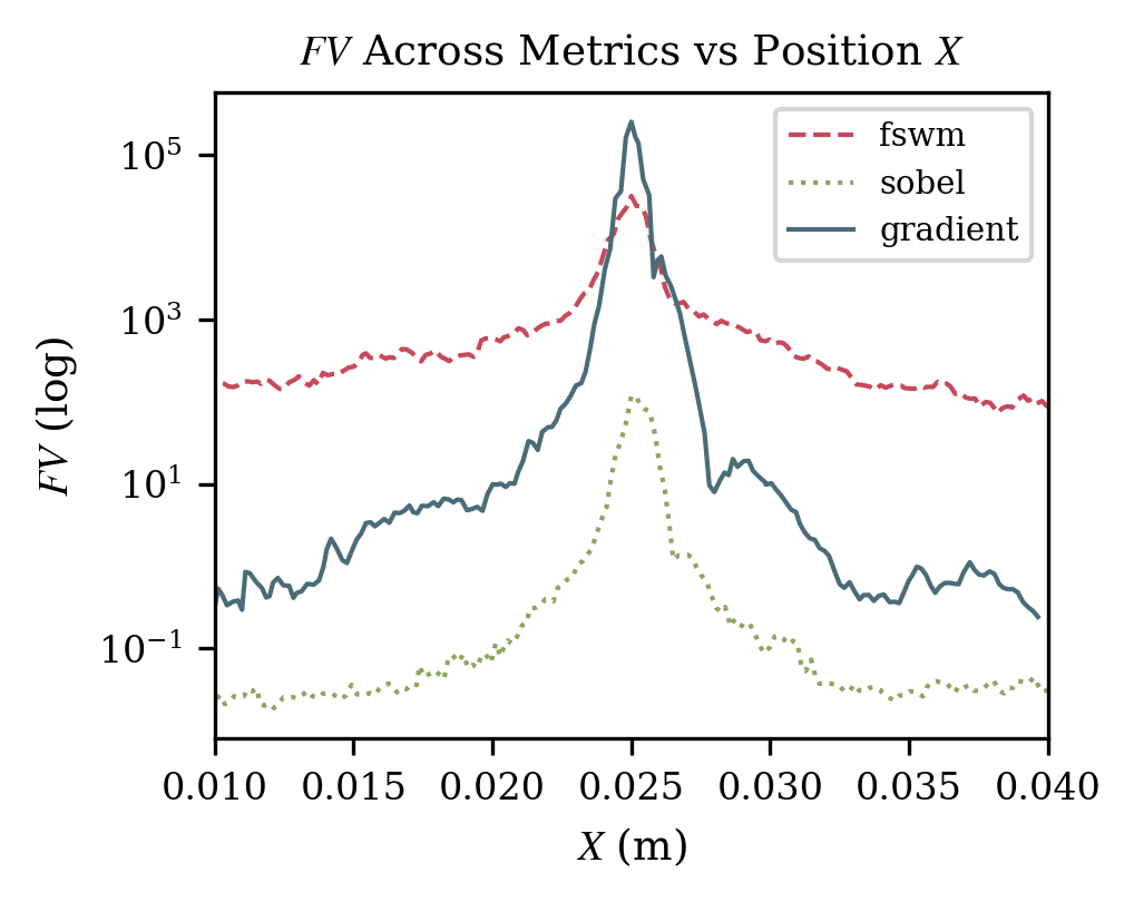
Slide 7 — The Core Problem: Metrics Vary Wildly in Scale

• FV magnitude depends on surface texture (rough steel ≫ smooth carbon fiber) and on the chosen metric
• Direct velocity control on raw FV → constant recalibration; impractical
• Figure: FV across FSWM / Sobel / SG on steel spans orders of magnitude (note: log scale)

---

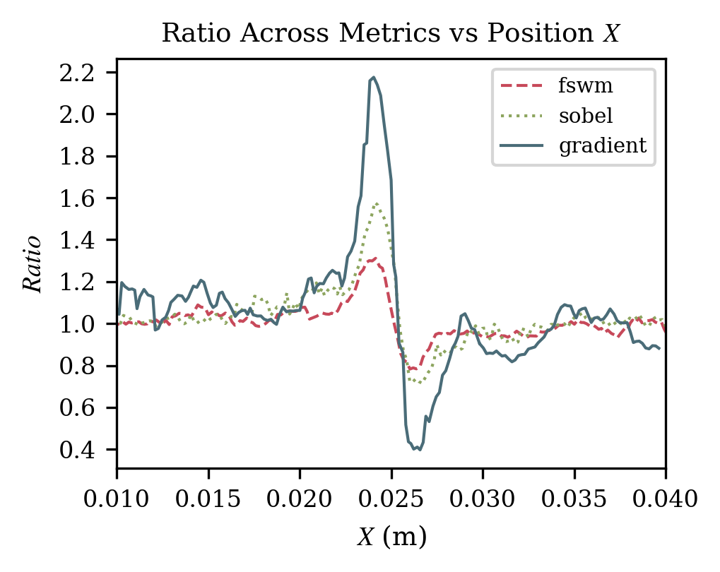
Slide 8 — The Ratio Insight

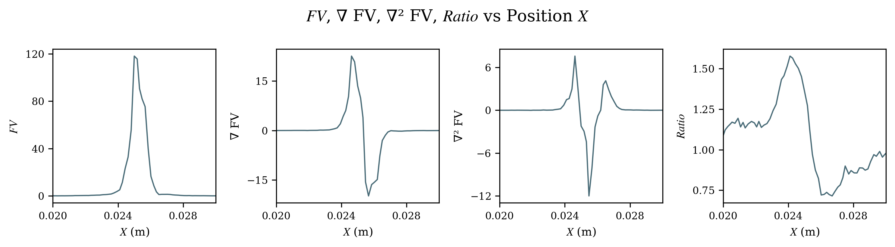
• Instead of raw FV, use the sign of derivatives + a ratio formulation:
  • $\nabla FV[t]=FV[t]-FV[t-1]$
  • ${\nabla }^{2}FV[t]=\nabla FV[t]-\nabla FV[t-1]$
  • $r[t]=FV[t]/FV[t-1]$
• Derivative signs are consistent across metrics → reliable coarse/fine mode switching
• The ratio compresses the dynamic range to a narrow band (r < 10) → one set of parameters works across metrics & materials

---

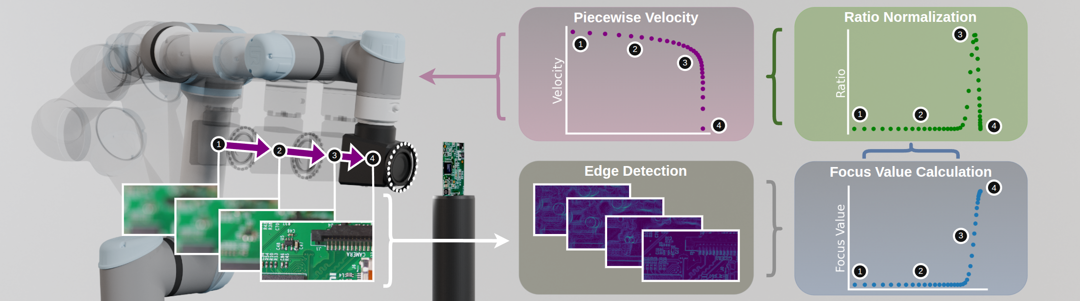
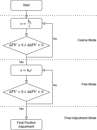
Slide 9 — The Control Algorithm

• Nonlinear velocity control (not discrete position steps) → smooth, responsive robot motion
• Three phases:
  • Coarse mode ($\nabla FV>0,{\nabla }^{2}FV>0$): $v=k_v/r[t]$ → low ratio far away = high velocity, fast sweep
  • Fine mode ($\nabla FV>0,{\nabla }^{2}FV<0$): $v=k_{v}r[t]$ → velocity decreases near peak for precision
  • Stop / final correction ($\nabla FV=0$): settle on stored max-FV position, correct overshoot
• $k_v$ = single unitless gain balancing speed vs. safety
• Starts unidirectional from the far end of the FV curve

---

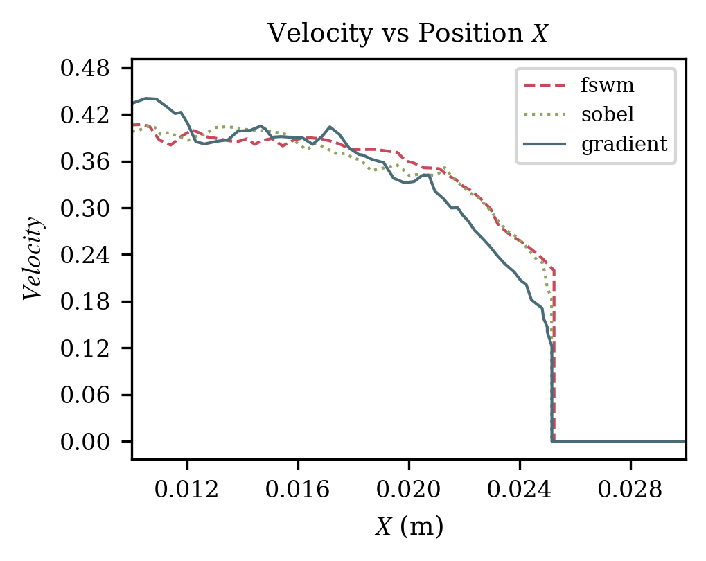
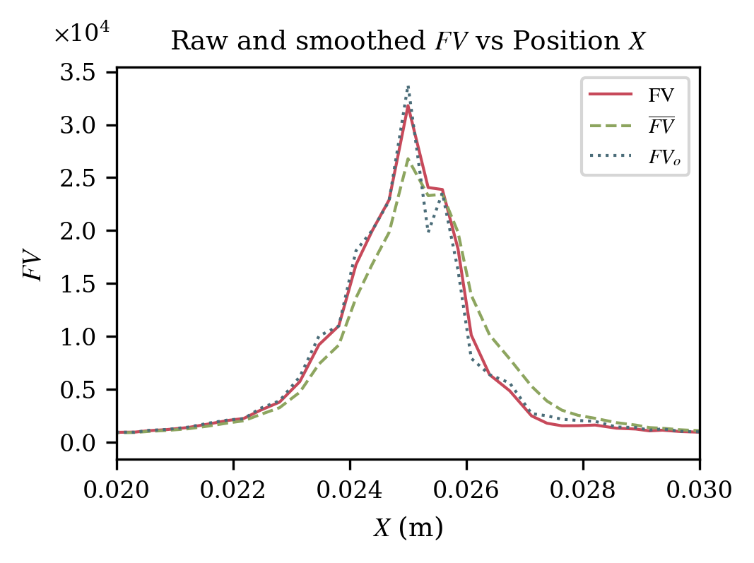
Slide 10 — Handling Noise: DEMA Smoothing

• Surface variation, robot motion, illumination, and sensor noise corrupt raw FV → noisy ratio/derivatives
• Apply Double Exponential Moving Average (DEMA): $FV=2\overline{FV}-\overline{\overline{FV}}$
• Reduces lag vs. plain EMA, preserves the location of the optimal FV
• Velocity profiles stay consistent across metrics without retuning

---

Slide 11 — Experimental Setup

• UR5e manipulator + eye-in-hand imaging: Sony IMX477 sensor, macro lens, addressable LED ring
• Magnification 0.18×, ~30 cm focus distance, 30 fps @ 1080p
• ROS2 + MoveIt2 Servo converts real-time velocity commands → joint trajectories
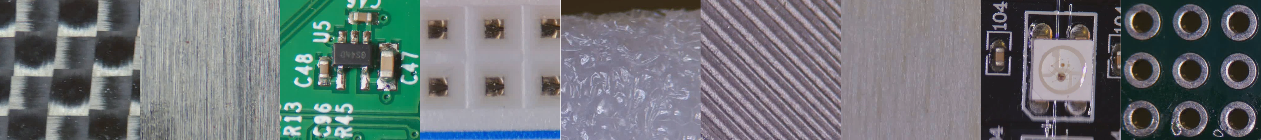
• 9 materials spanning texture/reflectivity: carbon fiber, unpolished steel, PCB, breadboard, foam, PLA, wood, LED strip, solder board
• Benchmark: Exhaustive Hill Climb (EHC) at constant velocity; both use identical fps, start position, distance; ratio $k_v=0.4$, EHC at half

---

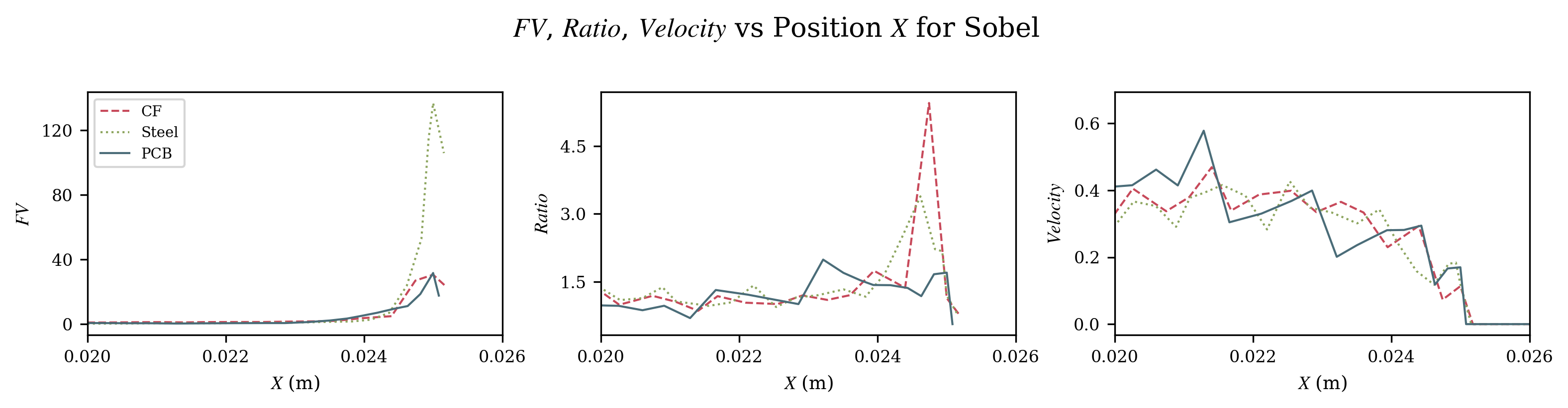
Slide 12 — Results

• Time: > 75% improvement over EHC across all materials and all metrics (~5–6 s vs. ~28–30 s)
• Accuracy:
  • Within 2 mm: breadboard, carbon fiber, foam, PLA (near robot’s absolute position limit)
  • Within 4 mm: LED strip, PCB, steel, wood, solder board
  • Max error: FSWM 1.99 mm, Sobel 3.69 mm, SG 2.97 mm; averages 0.85 / 1.56 / 1.32 mm
• Ratio bound: $r[t]<10$ across everything → compresses FV range by > 90%

---

Slide 13 — Impact of Material Characteristics

• Convergence speed is largely insensitive to surface appearance (uniform >75% time gain)
• Accuracy depends more on surface finish than on metric choice:
  • Reflective / low-texture (steel, LED strip, solder, wood) → weaker gradients → larger error
  • Strong intensity variation (carbon fiber) → stronger gradients → better accuracy
  • Textured + low-reflectivity (breadboard, foam, PLA) → clearest focus ratios
• DEMA keeps performance robust despite noise; ratio bounds instability across huge FV swings (e.g. SG FV spans 278 → 2.8×10⁵, yet r < 10)

---

Slide 14 — Conclusion & Future Work

• Ratio-based autofocus reliably works across multiple focus metrics and diverse materials with no recalibration
• Compressing FV into a bounded ratio is the key to robustness in dynamic inspection environments
• Validated on real hardware (UR5e + IMX477 + macro lens) under realistic cycle-time/reachability limits
• Future work: noise reduction for smoother ratio & tunable velocity profiles — especially on smooth/specular surfaces
• Thank you / Questions

---

Figure inventory (from the paper)

Slide	File	Paper caption gist
1, 3	new_system_image.png	UR5e + IMX477 + macro lens setup, FV curves along principal axis
5	algo_render.png	Autofocus control loop; 4-region velocity response
7	fv_comparison_log.png	Log-scale FV across FSWM/Sobel/SG on steel
8	ratio_comparison.png	Ratio narrows dynamic range across metrics
8	FV_dFV_ddFV.png	FV, ∇FV, ∇²FV, ratio vs. position
9	ratio_paper.png	Control-logic flowchart
10	smoothed_vel.png	Velocity profiles across metrics
10	fv_triplet.png	Raw vs. DEMA-filtered FV
11	coupon.PNG	9 test materials
12	results_sobel.png	FV / ratio / velocity for CF, steel, PCB

Tables (not images): Table I time performance, Table II position accuracy, Table III max ratio vs. FV — recreate as slide tables or pull the headline numbers (Slide 12).